


Basener, Sanford Defend Paper Critiquing Fisher’s Theorem, II
Bill Basener and John Sanford recently critiqued Fisher’s Theorem, a long-trusted model for neo-Darwinism. Two evolutionary geneticists responded. Here is Part II their counter-response. Go here for Part I.
Defending the validity and significance of the new theorem “Fundamental Theorem of Natural Selection With Mutations, Part II: Our Mutation-Selection Model
– Bill Basener and John Sanford
Joe Felsenstein and Michael Lynch (JF and ML) wrote a blog post, “Does Basener and Sanford’s model of mutation vs selection show that deleterious mutations are unstoppable?” Their post is thoughtful and we are glad to continue the dialogue. We previously wrote a first part of a response to their post, focusing on the impact of R. A. Fisher’s work. This is the second part of our response, focusing on the modelling and mathematics. Our paper can be found at: https://link.springer.com/article/10.1007/s00285-017-1190-x
First, a short background on our paper:
The primary thesis of our paper is that Fisher was wrong, in a fundamental way, in his belief that his theorem (“The Fundamental Theorem of Natural Selection”), implied the certainty of ongoing fitness increase. His claim was that mutations continually provide variance, and selection turns the variance into fitness increase. Central to his logic was that collectively, mutations have a net zero effect on fitness. While Fisher assumed mutations are collectively fitness-neutral, it is now known that the vast majority of mutations are deleterious. So mutations can potentially push fitness down – even in the presence of selection.
Additionally, we provided a new mathematical model for the process of mutation and selection over time, which comes in an infinite population version and a finite population version. The infinite population version uses a classical differential equations mutation/selection framework, with multiple reproducing subpopulations and mutations occurring between subpopulations, but incorporating a probabilistic distribution for mutation effects. The finite version is obtained by adding the constraint that any subpopulation with less than one organism is assumed to have no members.
Our model is backed by a literature review in Section 2 of our paper (covering 9 pages with 71 citations), with Section 2.2 discussing previous infinite populations models and Section 2.3 focusing on finite ones. Our model is new in that it includes an arbitrary distribution of mutational effects, and we do not assume mutations are 50/50 beneficial /deleterious (as did Fisher), and we did not assume that all mutations have the same fixed effect (as with Lynch’s finite population models).
Part II: Our Mutation-Selection Model:
Regarding our model, JF and ML describe it as follows:
“Basener and Sanford show equations, mostly mostly taken from a paper by Claus Wilke, for changes in genotype frequencies in a haploid, asexual species experiencing mutation and natural selection. They keep track of the distribution of the values of fitness on a continuous scale time scale. Genotypes at different values of the fitness scale have different birth rates. There is a distribution of fitness effects of mutations, as displacements on the fitness scale. An important detail is that the genotypes are haploid and asexual — they have no recombination, so they do not mate.” – Felsenstein and Lynch
This is an accurate description of our infinite population model. However, as we shall discuss shortly, they do not address our finite population version.
As a first minor point of correction, our equations are not taken from the cited paper by Claude Wilke. The Wilke paper is a nice review article, showing that two separate but significant lines of research (classic population genetics mutation-selection models and the Quasispecies or Replicator equations used in virus evolution) are mathematically equivalent, but no new equations are provided. Background support for our model is provided in Section 2, which as mentioned above is 9 pages in our paper and has 71 citations. The first-principles derivation of our infinite model, from standard population modeling principles, is given in Section 3.1 and the only previous model referenced in that section is the “special example” of Fisher’s theorem given in Crow and Kimura. The equations that JF and ML say we took from the Wilke paper were used (in equivalent mathematical forms) to prove a version of Fisher’s FTNS in Population Genetics by Hamilton (p.204), in An Introduction to Population Genetics Theory by Crow and Kimura (p. 10), and in The Mathematics of Darwin’s Legacy by P Schuster (p. 39).
In their analysis of our infinite model, JF and ML correctly point out that our model is haploid and asexual. This is true, and is the correct setting for our analysis of Fisher’s FTNS, and is the format used by Crow and Kimura, by Hamilton, and by P Schuster cited above. (The Crow-Kimura model is presented from a classical haploid asexual mutation-selection population genetics model while the Schuster Chapter motivates using a Replicator Equation; hence our citation of Wilke showing these two historically relevant lines of work are mathematically equivalent.) Lynch’s 1990 paper Mutation load and the survival of small populations (1990) similarly begins with a model focusing on asexual reproduction, and his model was extended to populations with sexual reproduction in Mutational meltdown in sexual populations (1995), where he showed results which “indicate that mutation accumulation in small, random-mating monoecious populations can lead to mean extinction times less than a few hundred to a few thousand years.” To the extent that JF and ML urge caution about using our model to make conclusions regarding sexual populations, we certainly agree. To any extent they dismiss our model because it is for asexual haploid populations, we disagree: this is the standard setting for Fisher’s FTNS, and is a natural simple case for first work that should be followed up with asexual models for extension to asexual populations which were not addressed in our paper.
JF and ML raise a question in the title of their post, “Does Basener and Sanford’s model of mutation selection show that deleterious mutations are unstoppable?” We do not actually make this claim, and this question is not directly addressed in our paper – we show Fisher’s claim of certain fitness increase is false due to mutation effects, and then give a model (with a finite and infinite version) and associated theorem that facilitates studying under what conditions fitness increases or decreases. We provide numerical simulations using the net-neutral-mutational-effect assumption inline with Fisher that shows fitness increase, and a simulation using the net-deleterious-mutational-effect from Kimura that undergoes continual fitness decline to demonstrate the importance of Fisher’s reliance on net-neutral mutational effects. Our paper provides a tool to better understand selection in the presence of deleterious mutations (actually more than that since we incorporate beneficial ones too), but does not pose any general answers for real biological populations other than saying they can go up or down. We are convinced that there is a very wide parameter space where fitness should be expected to decline, as ML has reported in many of his papers. The question of what parameters are required for equilibrium or continuous fitness gain is a subject we hope to address in the future.
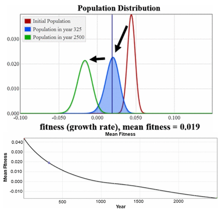
A focal point for JF and ML is our numerical simulation presented in Section 5.4. All of our simulations use our finite population model. The simulations in 5.1-5.3 either omit mutations or use a symmetric Gaussian distribution which is what Fisher considered for mutational effects, and the simulation in Section 5.4 uses the Gamma distribution for mutational effects from (Kimura 1979) with some beneficial ones added. The result is a fitness distribution for the population that declines steadily down through negative values, shown below.
Felsenstein and Lynch remark:
“…in their final case, which they argue is more realistic, there are mostly deleterious mutations. The startling outcome in the simulation in that case is their absence of an equilibrium between mutation and selection. Instead the deleterious mutations go to fixation in the population, and the mean fitness of the population steadily declines.”
They are correct in their description of the outcome. They find this result ‘startling.’ If this result were output from an infinite population it would be extremely startling; we provide a proof in Section 4 (Analytic Solutions) that the infinite version of our model goes to mutation-selection equilibrium. This is a classic result in this class of mutation/selection models. To explain the difference between output from our finite and our infinite models, we provide the following video: (https://www.youtube.com/watch?v=bBb4jPmctFk, The infinite model is on the left and goes to the guaranteed mutation–selection balance equilibrium while the finite one does not. All parameter values are equal.)
The two versions of our model are described in Section 3:
“The model can be treated as an infinite population model using the differential equation in Eq. (3.2), or as a finite population model when any subpopulation with less than one organism is rounded down. Thus, we use the first principles approach to modeling from the previous infinite population models, but incorporate the flexibility of the previous finite ones.”
We also describe the finite models in Section 5:
“To remain biologically realistic, we assume a finite population: any subpopulation Pi that contains less than some fraction of the population is assumed to contain zero organisms. For the numerical simulations, we set Pi=0 whenever Pi is less than 10−9 of the total population. This approximates a total population of 109 and eliminates any subpopulation with less than a single organism. The only case where this made an observable difference was Sect. 5.4. In that case, without the finite-population condition subpopulations remain viable even when they contain less than a fraction of an organism. As a result, extremely small, biologically nonsensical, populations control the observed results and obscure the effect of mutations on the population as a whole.”
In Section 4 we provide the formula for the mutation-selection equilibria for the infinite model and discuss the role of the infinite assumption:
“The sole equilibrium solution is the P=0, and all other solutions will be asymptotic to the eigenvector corresponding to the largest eigenvalue of W. By treating the system as a differential equation, we are implicitly assuming an infinite population; in this model, each Pi will be non-zero positive, but can be arbitrarily small. … These systems are considered infinite populations in part because each subpopulation Pi remains non-zero, regardless of how small Pi is compared to the total population. In the numerical simulations of Sect. 5, we address this be setting any subpopulation with sufficiently small fraction of the total population to zero.”
The theorem and accompanying formula provided in Section 4 is a classic result in mutation-selection models (see Burger 1989). It can be used to prove mathematically that our model is not an infinite model. The simulation in the accompanying video above shows the equilibrium and asymptotic eigenvector for the matrix W. If our model were an infinite model, it would have to be asymptotic to this same equilibrium (since the finite and infinite models in the video have the same matrix W), but it is not. Thus, our finite model is not an infinite model via proof by contradiction (assuming one trusts the output shown in the video).
The role of the finite assumption and its implications for mutation-selection balance are again described in the first paragraph to Section 3:
“In mutation–selection population models, as described in Sect. 2, there is a balance between the downward effects of deleterious mutations and upward effect of selection that balances out in infinite population models but not in finite population models. Our main theorem, Theorem 2, provides the rate of change of mean fitness into two terms, the first being the genetic variance and the second being a decrease in fitness from mutations, and the two are not equal.”
Not only is the role of the finite assumption pivotal in our paper, our main theorem (FTNSWM) provides insight into when fitness is increasing versus decreasing even when you do not have a guaranteed global attracting equilibrium. (Our theorem is exact for infinite populations and approximate for finite ones.)
Here is the analysis from JF and ML on why the population in our simulation from Section 5.4 experiences continual decrease:
“Why does that happen? For deleterious mutations in large populations, we typically see them come to a low equilibrium frequency reflecting a balance between mutation and selection. But they’re not doing that at high mutation rates!
The key is the absence of recombination in these clonally-reproducing haploid organisms.”
JF and ML ascribe the continual decline in fitness to the asexual haploid reproduction model and high mutation rates. The infinite asexual haploid reproduction model is mathematically guaranteed to go to equilibrium, so it seems counter-logical for them to use this to explain the lack of equilibrium if they believe that ours is an infinite population model.
Their comments on realistic mutation rates are absolutely important, and conclusions extending our model about general populations need to be done using a proper, rigorous, thorough exploration of parameters including mutation rates. But the mutation rates are not causing the ongoing continual decline; the infinite model with these same rates goes to mutation-selection equilibrium with mean fitness of 0.039 as shown in the video above.
JF and ML continue by putting parameters from our model through “the usual calculations of the balance between mutation and selection” (their words). But these do not apply because they are not derived from our model, but generally derive from infinite models – often considering a single mutation in isolation. Moreover, if our model results deviate from the usual calculations, it makes our model new, possibly interesting, but not wrong. (Again, we believe a proper evaluation on parameters including mutation rates should be done if general conclusions are to be drawn from our model. It is valid to evaluate our model either by evaluating the assumptions in its derivation or by comparing results to physical measurements, but not to challenge the model because it disagrees with other models.)
Their usual calculations for balance and selection assume our selection coefficient is “around 0.001”. But we do not have a fixed selection coefficient. We use a probability distribution to model mutational effects (specifically the Gamma distribution from Kimura 1979) with selection occurring as competition between different fitness, which is far more realistic than a single selection coefficient. The mean change in fitness in this distribution is 0.001, but most mutations will have an effect less than this value because the Gamma distribution is skewed (its median is less than its mean). As stated in Mutational meltdown in sexual populations (1995), the value of a selection coefficient (impact on fitness by a mutation) greatly impacts the decrease in fitness from mutation accumulation:
“It is now well established that mutations with small, but intermediate, deleterious effects cause the most cumulative damage to populations (Kimura et al. 1963; Gabriel et al. 1993; Charlesworth et al. 1993). Mutations with very large effects are eliminated efficiently by selection and have essentially no chance of fixation, whereas neutral mutations have no influence on individual fitness. The diffusion theory developed by Lande (1994) suggests that the value of s that minimizes the time to extinction, that is, that does the most damage, is s* = 0.4/Ne. T”
Our model is a finite model with mutations occurring probabilistically across a realistic distribution of effects on fitness, which is a significant deviation from most previous models. We use a novel method for finite populations, which enables us to use the rigorous derivation of standard mutation-selection infinite population models, enables us to apply the formula for change in fitness due to selection (upward force) vs mutation (downward force) proven in our main theorem, and enables us to use an arbitrary probability distribution for mutational effects.
JF and ML comment:
“So there is really nothing new here.”
And then conclude with statements about what would change in the output from our model if certain changes were made.
“If Basener and Sanford’s simulation allowed recombination between the genes, the outcome would be very different — there would be an equilibrium gene frequency at each locus, with no tendency of the mutant alleles at the individual loci to rise to fixation.
If selection acted individually at each locus, with growth rates for each haploid genotype being added across loci, a similar result would be expected, even without recombination. But in the Basener/Stanford simulation the fitnesses do not add — instead they generate linkage disequilibrium, in this case negative associations that leave us with selection at the different loci opposing each other. Add in recombination, and there would be a dramatically different, and much more conventional, result.”
Clearly, we believe that JF and ML misunderstand our finite model and its implications. However, and this is significant, we agree with them regarding the answer to the question they pose in the title of their post, Does Basener and Sanford’s model of mutation vs selection show that deleterious mutations are unstoppable?. Our paper does not show that they are unstoppable, and does not try to. It is significant that JF and ML raise this question.
Our paper does show that the buildup of deleterious mutations can be significant, but this was known before; our result in the simulation in Sec 5.4 is consistent with results from Lynch. Our paper shows that this fitness decline occurs in the context of Fisher’s model when realistic factors (realistic mutation distribution and finite population) are incorporated. It does show that Fisher’s conclusion about application of his FTNS is false, and in a way so fundamental that his FTNS gives no real support for the Neo-Darwinian Theory. We provide a new model and new analytic tools that can be used to examine whether fitness is going up or down, and these can incorporate realistic factors in ways not previously considered.
Application of any model to real biological populations is a big undertaking, and must be done with impartial use of the ranges for previously published ranges for parameter values (such as mutation rates and mutation effects), and a consideration of the explicit and implicit assumptions in the model derivation and their relevance to reality.
A good example of examining competing hypothesis using ecological economics population models I (Bill B) developed for collapse in ancient human civilizations is given in The slow demise of Easter Island: insights from a modeling investigation. This is an extremely hotly debated topic with intelligent and qualified camps with differing views, including anthropologist Terry Hunt from the University of Hawaii who has spent his career studying Polynesian-type islands, and the high-profile Jared Diamond from UCLA with his Guns, Germs, and Steel approach. You can read some of the online debate here, here, and here. And if you want to see academic discussion gone really really bad, read this paper. (See my very measured response to a newspaper interview here. I am not a fan of jumping to conclusions regardless of prior belief.) But the real point is, despite the amount of personal views and emotion, The Slow Demise paper is a good model for testing population models, basing conclusions on thorough background exposition, examination of the derivation and components of a model, and then examination of the variety of possible outcomes.
Conclusions:
- R. A. Fisher was one of the three founders of population genetics, and is considered by many to be the principle founder. His FTNS theorem has been considered a significant and rigorous support for the Neo-Darwinian Theory.
- Fisher’s theorem in fact does not provide support for the Neo-Darwinian Theory. The upward pressure of selection on fitness cannot be realistically considered apart from the downward effect of mutations.
- JF and ML state that our paper does not show that deleterious mutations are unstoppable. We agree; our paper shows what can happen, not what must happen. Conclusions about what our model predicts, given biologically realistic parameters, is a separate undertaking.
- JF and ML gave an accurate description of our infinite model, but misunderstood the finite model, apparently because it is a new form of finite model.
- Our finite model is constructed in a new manner. We can prove mathematically that this is not an infinite model. Novel attributes include the use of a realistic distribution of mutational effects, use of classic form for instantaneous rates of change in a finite model, and analysis with our new FTNSWM Theorem.
- JF and ML gave analysis using standard computations from infinite models and with selection happening separately at each locus, which is not relevant to our model because ours is not an infinite model.
- JF and ML conclude from their standard computations that “there is really nothing new here.” It is ironic that they fail to recognize our new finite model, and then declare that there is nothing new.
- They conclude by claiming that if our model were modified to include recombination, the result would be more conventional. We do not think it is possible to know the outcome of a model without building it. This work will follow.
In short, we agree with JF and ML that our paper does not show that deleterious mutations necessarily result in declining fitness. However, we have clearly falsified the converse claim, which is that genetic variance plus selection necessarily result in increasing fitness.
If Joe F and Michael L write a response, we politely request that they provide quotes from our paper that support their claims that we argue that fisher’s FTNS “is the basis for all subsequent theory in population genetics.” (Full sentence: “This is presented as correcting R.A. Fisher’s 1930 ‘Fundamental Theorem of Natural Selection’, which they argue is the basis for all subsequent theory in population genetics.”) We also invite them to clarify if our paper claims that “deleterious mutations are unstoppable” as seems to be implied in the title of their article, and provide quotes from the paper if they believe we support that premise.
Final Comment from Basener: Please forgive this minor soap box issue of mine, but I want to encourage careful interpretation of mathematical models, especially regarding assumptions and parameters that are not fully known. Mathematical models are not reality. Fisher made a mistake in his assumptions applying his theorem, and it led to some bad conclusions for 50-100 years. Here is a quote from the third paragraph of Section 2 of our paper:
“Every model is only an approximation of some isolated subset of reality, and each model is only useful insofar as it: (1) includes the variables and rules to be studied and: (2) the rules governing change in the model accurately approximate the most important factors affecting change in reality. Simple rules make a model more mathematically tractable, but at the cost of utility as a useful model of reality. The general goal is to have rules that are as simple as possible, and yet capture all the driving factors contributing to the phenomena to be studied. In using a model to make general statements about behavior in reality, it is essential to consider the built-in assumptions implicit in the structure of the rules in a model.”
Here is a related quote from Okasha, that J-Mac posted recently:
“It is clear that population genetics models rely on assumptions known to be false, and are subject to the realism / tractability trade-off. The simplest population-genetic models assume random mating, non-overlapping generations, infinite population size, perfect Mendelian segregation, frequency-independent genotype fitnesses, and the absence of stochastic effects; it is very unlikely (and in the case of the infinite population assumption, impossible) that any of these assumptions hold true of any actual biological population. More realistic models, that relax one of more of the above assumptions, have been constructed, but they are invariably much harder to analyze. It is an interesting historical question whether these ‘standard’ population-genetic assumptions were originally made because they simplified the mathematics, or because they were believed to be a reasonable approximation to reality, or both. This question is taken up by Morrison (2004) in relation to Fisher’s early population-genetic work.” —Samir Okasha 2006/2012
Update 3/20/18: Joe Felsenstein has issued a response to two of three points at The Skeptical Zone.